Have you ever had a large amount of data in Excel and need an easy way to visualize your data for trends, priorities, or other measures? Sometimes it’s necessary to be able to get information at a quick glance without sifting through every item.
What is Conditional Formatting?
Conditional Formatting will automatically format cells based on a condition that you have pre-determined. It makes it easy to highlight specific data by using color scales, icon sets, or your own specified formatting. There are tons of combinations that you could use with Conditional Formatting and we’re going to go over a few examples.
Apply Conditional Formatting Based on a Date Range
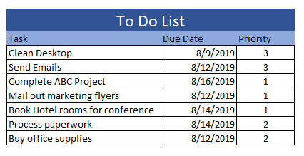
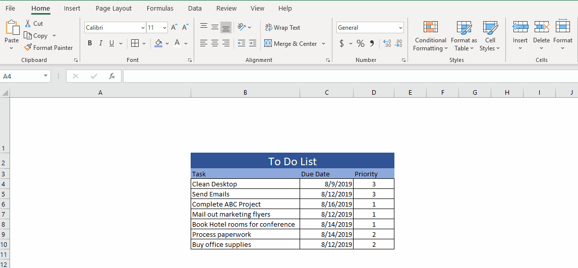
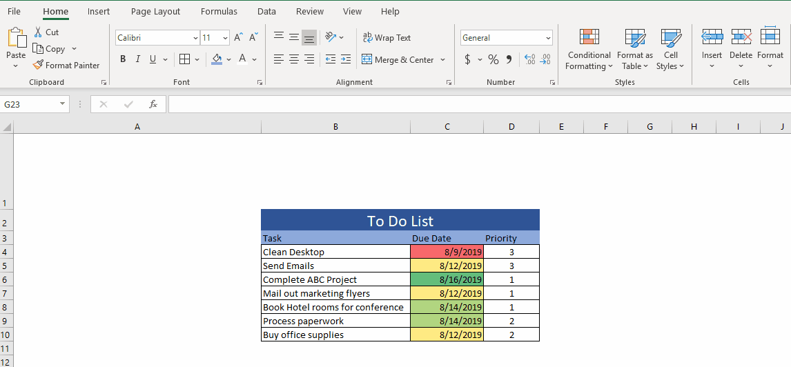
Let’s start with a simple To-Do list made in Excel. The second column holds due dates in mm/dd/yyyy format. Let’s apply conditional formatting to highlight the due date column based on how close the date is to today being red and the furthest due dates to Green, all others will be Yellow.
See the before and after pictures of this list:
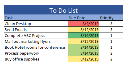
Now let’s set a Conditional Formatting to color the dates in that column with the closest dates to today being red and the furthest due dates to Green, all others will be Yellow. Here are the steps to take.
- Highlight the cells that you want to apply the conditional formatting to.
- Select Conditional Formatting located in the Styles section of the Home Ribbon.
- Choose Color Scales.
- Apply whichever color scale you would like to use.
Apply Conditional Formatting Based on a Number
Let’s take the same To-Do list and make similar conditional formatting using the priority column. This time I would like to place an icon in the field based on the priority number. Here are the steps to do this:
- Highlight the cells that you want to apply the conditional formatting to.
- Select Conditional Formatting located in the Styles section of the Home Ribbon.
- Choose Icon Sets.
- Apply whichever icon set you would like to use.
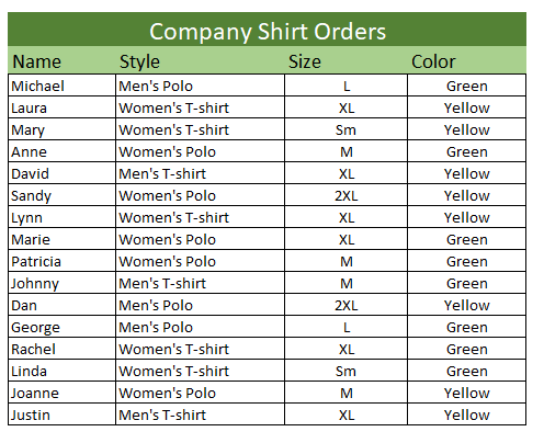
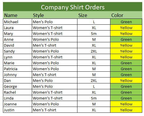
Apply Conditional Formatting based on Text
This third example is a bit different. This time we are going to specify our formatting based on a color named in the excel spreadsheet. See the Before and After:
Here are the steps:
- Highlight the cells that you want to apply the conditional formatting to.
- Select Conditional Formatting located in the Styles section of the Home Ribbon.
- Choose Highlight Cells Rules.
- Choose Text That Contains
- In the first box type the text that you want to be formatted a specific way.
- In the second box choose Custom Format.
- Select the formatting that you would like.
- Click Ok. Click Ok again.
Conditional Formatting allows you to visualize your data in many ways. There are many applications that you could apply this to! Try it out in a blank spreadsheet!
About Harbor Computer Services
Harbor Computer Services is an IT firm servicing Southeastern Michigan. We work exclusively under contract with our clients to provide technology direction and either become the IT department or provide assistance to the internal IT they already have. We have won many awards for our work over the years, including the worldwide Microsoft Partner of the Year in 2010. We’re the smallest firm to have ever won this most prestigious award. Most recently we were recognized as one of the top 20 visionaries in small business IT by ChannelPro Magazine (2015). And in 2016 as the top Michigan IT firm for Manufacturing. There are a few simple things that make Harbor Computer Services the best choice for your business. •We are Professionals •We are Responsible •We are Concerned About The Success of Your Business


